Bullwhip and demand amplification

One weekend promotion in the shop, and two weeks later the team at the plant is working overtime. Customers did not suddenly eat twice as much chocolate: the shelf simply emptied, the shop ordered double to be safe, the wholesaler topped the order up, and the manufacturer already sees a rising trend in its data and revs up the production plan. This is the crack of the whip: a small movement at the handle lands as a big blow at the end. Let’s look at what this phenomenon is, what it costs, and which map makes it visible.

The bullwhip (Forrester) effect: demand swings amplify the further upstream you go from the end customer. Demand amplification mapping makes it visible.

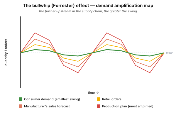
Figure 1 — the demand amplification map on the classic example of a well-known chocolate bar. The same demand at four levels: consumer demand fluctuates least, and going upstream (retail orders, the manufacturer’s sales forecast, the manufacturer’s production plan) the amplitude keeps growing. The curves “open up” — this is the bullwhip effect.

Who is this for?

This article is for those who work with the schedule, the inventory or the orders: production planner · plant and shift supervisor · process technologist · logistics specialist · supply chain analyst · buyer · Lean/CI specialist · process engineer.

Learning objectives

After reading this article you will be able to:

• explain what the bullwhip (Forrester) effect is, and why it makes flow harder;
• list the three questions the demand amplification map answers;
• walk through the six steps of building the map on one of your own products, with the right time horizon and unit of measurement;
• separate amplification caused by changeovers from amplification caused by inventory policy, and pick the right intervention for each;
• say when this map is not the right entry tool.

In brief

• Demand amplifies upstream. Consumer demand swings least, while at the upper levels of the chain (retailer, manufacturer’s forecast, production plan) the swing keeps growing.
• The greater the amplification, the harder the flow. The ideal is that every production stage works at the customer’s rate of demand, because that brings uninterrupted flow (heijunka, pull).
• The map is a quantity-against-time graph: it plots the batch sizes of a product at the stages of the process, and the inventory along the chain through time.
• It is used for three purposes: (1) showing the extent of amplification; (2) exposing the batch sizing and scheduling policies (quantity and timing); (3) checking the inventory decisions, since inventory is the buffer between demand and supply.
• Two kinds of amplification must be separated: the one caused by changeovers (batching), and the one caused by inventory or safety stock policy.
• Lean produces not only frequently but also regularly (say, the same day each week), and it avoids the “temptation to overproduce” while the set-up is in place.
• Data need: a one-month snapshot is often adequate, but 4–6 months gives a clearer picture; the time horizon must cover at least three batches at the longest manufacturing cycle.

Why it matters (the stakes)

Amplification is not a statistical curiosity but direct operational damage: it creates an unlevelled and interrupted schedule. That is exactly why it is an indispensable tool when mapping is extended along the supply chain: it exposes the demand fluctuations that wreck the schedule, and through this it makes three concrete problems measurable.

What amplification causes	How it shows up	What you can do about it
Unlevelled, interrupted schedule	you idle at times, you rush at others; frequent rescheduling	levelling to the customer rate (reducing mura)
Mismatch in order quantities	customer and supplier think in different quantities	aligning the ordering rules
Poor inventory control routines	a “better safe than sorry” buffer at every level	stating and reviewing the inventory policy

The greater the amplification, the harder it is to create flow, and the more unnecessary inventory waste sits in the chain. That is the stake: at every single level, amplification breeds inventory, rushing and unnecessary changeovers.

What is the bullwhip (Forrester) effect?

The bullwhip effect is the phenomenon where demand changes grow larger and larger the further you get from the original demand source, that is, from the end customer. The phenomenon was described by Jay Forrester (hence the “Forrester effect”); its everyday name is bullwhip: just as a small movement at the handle of a whip builds into a big crack at the tip, a small change in demand amplifies as it passes upstream in the supply chain.

The classic textbook example is a well-known chocolate bar (Figure 1): of the four curves of the same product, consumer demand fluctuates least, retail orders already swing more strongly, the manufacturer’s sales forecast even more, and its production plan the most of all. Going upstream, the curves “open up.”

What does the demand amplification map make visible?

The map makes the extent of amplification, the batching and scheduling policies, and the inventory decisions visible all at once. As a member of the detailed VSM toolbox (the seven tools of Hines and Rich), it is, alongside Process Activity Mapping, the most powerful technique: it shows why inventory exists at all, and it highlights the problems of the batch size and inventory policies adopted by either the customer or the supplier. The map answers three questions:

1. How great is the amplification as orders are passed upstream? The greater it is, the harder it is to encourage flow. The ideal is that all stages work at the customer’s rate of demand, bringing uninterrupted flow.
2. What are the batch sizing and scheduling policies? Quantity and timing must be examined together; this is how the reasons for excessive batches or lack of synchronisation can be explored.
3. Are the inventory decisions right? Inventory is the buffer between demand and supply; if there is synchronisation between demand and supply, inventories should be low.

How do you build the map?

In six steps: you identify the data collection points, select the product, decide the time horizon and the period for analysis, collect batch size and inventory data, and finally plot it. Most mistakes come from a badly chosen time horizon and unit of measurement, so pay particular attention to those.

1. Identify the stages at which you will collect data. The first is usually the actual customer demand; the subsequent ones are the major production stages or cells. Look out for inventory storage, and record data at and after each inventory location.
2. Select the product or part to be studied. Preferably the one for which you have already collected data for other maps (for example Process Activity Mapping); if there is none, select a representative part.
3. Decide the time horizon. It should include a minimum of three batches at the longest manufacturing cycle. (If, for instance, batches are made fortnightly at a press stage but assembly takes place every two days, then record three press batches over four weeks.)
4. Choose a “typical” period for analysis. Avoid rush and quiet periods; here the company’s record keeping system may constrain you.
5. Collect batch size and inventory data. A batch may take more than one day to produce; inventory can also be derived from the batch sizes as long as one accurate snapshot can be made.
6. Plot the data on a graph.

Two practical tips for data collection

Unit of measurement. Use a unit that fits the process: if, for example, a plastic moulding has a shot (raw material) weight of 50 g, then measure raw material purchases so that 50 g equals 1 unit. Do not collect from too many points. In some firms data could be collected from more than a dozen points, but be selective: three or four well chosen points will give you 99% of the information, with far less work and analysis time.

How to start tomorrow

Pick a product whose actual customer call-off you know. Designate three points: the customer order, an intermediate inventory location and your own production plan. Going four weeks back, write out the ordered and the produced quantities in the same unit of measurement, and draw them on one graph. If the amplitude of the three curves grows upstream, you have found the amplification, and the analysis can begin.

What do you read out of it?

Whether the swings come from changeovers or from inventory policy, because the two call for two different interventions. The map is powerful because it does not record the schedulers’ theoretical answers (how they make up the schedule), but allows discussion around what actually happens and how it can be improved.

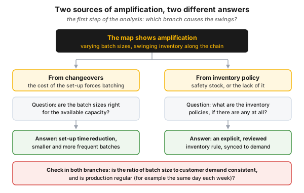
Figure 2 — the two sources of amplification and the answer to each. Batching that comes from changeovers is answered by set-up time reduction; amplification that comes from inventory policy is answered by an explicit and reviewed inventory rule.

• Separate amplification due to changeovers from amplification due to inventory policy. Changeovers lead to batching. The question is whether the batch sizes are appropriate in relation to the available capacity. For amplification due to inventory policy, ask what the policies are, if any.
• Look for variation in batch sizes. How consistent is the ratio of batch size to customer demand? From there, ask about the batch sizing policy. Watch out for the temptation to overproduce while the set-up is in place.
• Look for the regularity of batches. A Lean operation attempts to run products not only as frequently as possible, but as regularly as possible — say, the same day each week.

Where do you intervene in the supply chain?

In two kinds of place: in the co-ordination between companies and in the development inside individual companies. When you extend the mapping to suppliers and customers, two types of waste (and opportunity) are to be expected, and reducing the amplification also happens in these two bands.

Band of intervention	Where the waste arises	Typical intervention
Supply chain co-ordination	between companies	common quality standards, the same paperwork system, shared transport, inter-company communication methods (EDI)
Supply chain development	inside individual companies of the chain	dissemination of customer strategies (so suppliers can plan better), assistance in factory layout, set-up time reduction and the operation of internal kanban systems

Mapping with external companies calls for care and diplomacy: the methods are the same, but the team is wider. This is the point where the map yields the most insight, because a good part of the amplification arises at the boundary between companies.

How is it used in the process industry?

In continuous operation, amplification does not show up in “boxed” batches but in campaign lengths, tank policies and scheduling. If the supply chain forecast and the production plan swing strongly compared with relatively stable end-user demand, the plant is forced into frequent load and mode changes. The demand amplification logic suggests the same here: levelled production, aligned to the rate of demand (heijunka, reducing mura) gives a more stable flow.

Safety focus

The operational price of amplification is many transients: load changes, mode changes, start-ups and shutdowns. Start-up, shutdown and load-change states are elevated-risk operating states, because many parameters move at once and practised routine helps less than in steady operation. Reducing the bullwhip is therefore not only an inventory and cost question: a more stable, more predictable operation is also safer. In this way the map is indirectly a tool for making mura (unevenness) visible, and mura is one of the main sources of waste and risk (see the role of near-miss reporting in early warning).

Common mistakes

The pitfalls almost all start either from the map not recording reality, or from choosing the wrong intervention for it. Anti-pattern and correction in pairs:

• You accept the schedulers’ theoretical answer. You draw up the described planning logic instead of the actual data. Instead: the map is precisely about real operation, so put measured quantities on it.
• You do not separate the two sources of amplification. You blur changeover and inventory-policy causes together, and so reach for the wrong tool. Instead: first decide according to Figure 2, then choose the intervention (SMED or inventory policy).
• You overproduce while the set-up is in place. Convenient, but this is exactly what enlarges the batches and the amplification. Instead: size the batch to customer demand, not to the convenience of the set-up.
• You take too short a time horizon. A single week misleads, because the batch cycle does not even finish. Instead: at least three batches at the longest manufacturing cycle.
• You ignore regularity. You look only at frequency, not at the predictability of the rhythm. Instead: also examine whether the batch runs on the same day week after week.
• You see the bullwhip only as a supplier problem. You demand the ordering rules from others. Instead: look at your own forecasting and batching policy too, because a good part of the amplification arises there.
• You collect data on everything. You burn up the analysis time of a dozen measurement points. Instead: three or four well chosen points will give you 99% of the information.

When NOT to use it (the limits of the method)

When the pain point is neither inventory nor batch size. The demand amplification map is the sharpest tool for the wastes of overproduction and excess inventory; for other waste types another map of the VSM toolbox is the right entry point.

Situation	Why this is not the right tool	The right answer
The waste is at the level of the steps (motion, waiting, over-processing)	the map looks at quantity through time, not at the operational steps	Process Activity Mapping
The pain point is defects and customer service	the map says nothing about defect types	Quality Filter Mapping
One-off, non-repetitive production, with no meaningful batch cycle	there is nothing to follow across three batches	process-level mapping or standard work
There is no access to actual order and inventory data	a curve drawn from theoretical answers misleads	data collection first, even by recording it yourself
The question is the root cause, not the pattern of the fluctuation	the map answers the what and the where, not the why	root cause analysis, then a map to confirm the effect

Rule of thumb: the demand amplification map is strongest when inventory and schedule fluctuation are the problem in repetitive, batched or campaign-type production.

Take it home (keys)

• Draw the curves going upstream: if the amplitude grows from level to level, the bullwhip has become measurable, and you no longer have to argue over opinions.
• Separate first, intervene second: for a changeover cause the right step is set-up time reduction (SMED); for an inventory-policy cause it is stating and reviewing the rule.
• Look at your own back yard too: a good part of the amplification comes from your own forecasting and batching policy, not from the supplier’s.
• Three or four well chosen measurement points are enough, and the horizon should cover at least three batches at the longest cycle.
• Regularity is as much a goal as frequency: a Lean operation runs as frequently and as regularly as possible.
• Close with action: the map is the beginning of the debate about batch sizing, scheduling and inventory policies, not the end.

Self-test

1. What is the bullwhip (Forrester) effect, and at which point is the fluctuation greatest in the chocolate bar example?
2. The map shows swings. Which two sources must you separate, and which intervention belongs to which?
3. Batches are made fortnightly at a press stage and every two days at assembly. What time horizon should you choose for data collection, and why?

Answer key

1. Demand fluctuation amplifies more and more as you move upstream in the supply chain, away from the original demand source (the end customer). In the example the manufacturer’s production plan fluctuates most, and consumer demand least.
2. Amplification due to changeovers (the changeover leads to batching; the question is whether the batch size is appropriate for the available capacity, and the answer is set-up time reduction and smaller, more frequent batches), and amplification due to inventory or safety stock policy (the question is what the policies are, if any; the answer is an explicit, reviewed inventory rule).
3. Four weeks, because the horizon must cover at least three batches at the longest manufacturing cycle; here that is the press batch (fortnightly), so three press batches over four weeks.

How does this show up in digital practice?

The analysis of demand amplification does not stop at a hand-drawn graph: the same logic is realized digitally too. The mechanism differs, the principle is the same: the data does not have to be scraped together afterwards, it is recorded as it arises.

Principle	Digital implementation	What it delivers
Quantity as a function of time	automatic time-series collection of order, batch size and production quantity data	the curves come out by themselves, not from a separate data collection project
Inventory along the chain	continuous recording of tank, buffer and stock levels	the buffer is not an estimate but a measured time series
Load and mode change	e-log and shift handover: when, by how much and for what reason the load changed	the number and the cause of the transients are retrievable
Schedule deviation	plan versus actual per shift, deviation report	the unlevelled schedule becomes quantifiable
Batch regularity	analysis of the timestamps of batch starts	it becomes clear whether the batch really runs on the same day

The essence

Modern digital systems realize the same principles as the map drawn on paper: they make the development of quantity and inventory over time visible. If a system records and trends schedule deviations and load changes by itself, a live demand amplification analysis is at work in the background.

Connection to OPEREX (shift log)

To diagnose the amplification you have to know why the load or the operating mode changed: because of real demand, or because of an internal batching and inventory policy? The OPEREX shift log records the actual performance and mode changes (when, by how much and for what reason the load was raised or cut) with a timestamp. From this it can be reconstructed afterwards whether a swing followed the customer’s demand or was generated by the chain itself, which is exactly the separation the analysis calls for. On top of that, a levelled operation means fewer transient interventions, which is auditably traceable from the log, and is at once a cost, an inventory and a safety gain.

Terminology (HU / EN / JP)

Hungarian	English	Japanese / note
ostorcsapás-hatás	bullwhip effect	the everyday name
Forrester-hatás	Forrester effect	after Jay Forrester
keresletfelerősítési térkép	demand amplification mapping	the quantity-against-time graph
kötegméret	batch size	the main driver of amplification
átállás	changeover / set-up	段取り替え — causes batching (see SMED)
biztonsági készlet	safety stock	a source of amplification
kiegyenlítés, szintezés	levelling (heijunka)	平準化 — the direction of the solution
egyenetlenség	unevenness (mura)	ムラ — what amplification produces
vevői keresleti ütem	customer rate of demand	the rate of the ideal
jelzőkártyás húzórendszer	kanban	かんばん — the internal kanban system

A Japanese equivalent belongs only to the concepts of Toyota origin; the mapping tools are Western (UK academic) developments.

FAQ

What is the bullwhip (Forrester) effect?

The phenomenon where demand fluctuations amplify more and more the further you get from the end customer, going upstream in the supply chain. The manufacturer’s forecast and production plan show a far greater swing than actual consumer demand.

Why is the bullwhip effect bad?

The greater the demand amplification, the harder it is to create continuous flow, and the more unnecessary inventory accumulates in the chain. Amplification causes an unlevelled and interrupted schedule, and it brings to the surface mismatches in order quantities and poor inventory control routines. In continuous operation all this also means many transient mode changes.

What does Demand Amplification Mapping make visible?

On a quantity-against-time graph, the batch sizes of the product and the inventory at the stages of the process. It shows the extent of the amplification, the batching and scheduling policies and the inventory decisions, and it helps to separate amplification due to changeovers from amplification due to inventory policy.

How much data does the map need?

A one-month snapshot is often adequate, but a four to six month period gives a clearer picture. The time horizon must cover a minimum of three batches at the longest manufacturing cycle. As for measurement points, three or four well chosen ones give 99% of the information.

Which is the most powerful tool in supply chain mapping?

Process Activity Mapping and the demand amplification map. The latter shows why inventory exists at all, and highlights the problems of the inventory and batch size policies of either the customer or the supplier.

Related concepts

the detailed VSM toolbox · mura · the pull system · flow · SMED · kanban · muda · VSM

Next step

Once you can see the amplification, it is worth going on in this order:

1. the detailed VSM toolbox — the full mapping toolkit: which map is sharpest for which waste, and in what order to deploy them.
2. mura — the concept of unevenness and the logic of levelling; this is the actual answer to amplification.
3. SMED — set-up time reduction, that is, the concrete antidote to amplification caused by batching.

References / further reading

• Peter Hines & David Taylor: Going Lean. Lean Enterprise Research Centre, Cardiff Business School, 2000. — the practical handbook of the detailed mapping tools, including the method of the demand amplification map and the chocolate bar example.
• Peter Hines & Nick Rich: The Seven Value Stream Mapping Tools. International Journal of Operations & Production Management, 17(1), 46–64, 1997. — the canonical, published description of the seven detailed mapping tools.
• Jay W. Forrester: Industrial Dynamics. MIT Press, 1961. — the foundational work on supply chain amplification (the Forrester effect named after him).
• John Bicheno & Matthias Holweg: The Lean Toolbox. PICSIE Books. — the further reading explicitly recommended by the source material on applying the mapping tools.